Introduction

Every chemical process depends on hundreds of variables – including temperature, pressure, flow, and composition – that must be kept within a narrow operating window to run safely and profitably. Manual operation cannot keep pace with that demand, especially as processes grow larger and more complex. Control loops fill that gap: they measure process conditions, compare them to a target, and automatically adjust the process to hold that target. Designing a control loop that performs reliably, however, takes more than selecting a controller and setting it to run. It requires a clear control strategy, the right instrumentation, and tuning parameters matched to the process. This article covers the core principles behind designing and tuning control loops for automated operation of chemical processes.

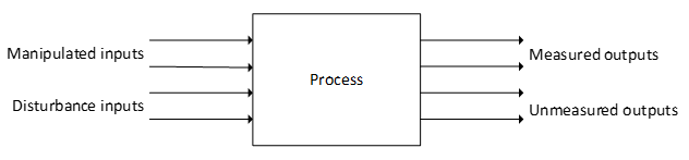
Figure 1 shows a conceptual process block diagram of a chemical process where inputs are classified as manipulated or disturbance and outputs as measured and unmeasured.

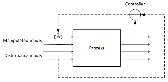
Process automation requires the use of measurements of process outputs or disturbance inputs to make decisions regarding the proper values of manipulated inputs. This is the main purpose of a control loop, as shown in Figure 2; the measurements and control signal are represented as dashed lines.

Defining the Control Strategy

The main objective of process automation is to define a control strategy. The definition for a control strategy consists of formulating or identifying the following:

• Control objective(s)
  • The initial step to develop a control strategy. A process unit consists of several different unit operations that are generally controlled separately. It is very common that every unit operation may have multiple and sometimes conflicting control objectives.
• Input variables
  • Can be classified as manipulated or disturbance variables. The manipulated input can be adjusted by the process operator and/or the control system. On the other side, the disturbance input directly affects the process output and cannot be adjusted.
• Output variables
  • These variables can be classified as measured and unmeasured.
• Constraints
  • All chemical processes have operating constraints classified as hard or soft. An example of a hard constraint is a minimum/maximum operating pressure (i.e., a pressure regulator operates between fully open or fully closed). An example of a soft constraint is a distillation column product purity (i.e., could temporarily be exceeded but will not stop the operation and the control loop will work to pull it back down).
• Operating characteristics
  • Classified as continuous, batch, and semi-batch. Continuous processes operate for long periods of time at relative constant operating process conditions before being shut down for scheduled maintenance. Batch processes generally operate for a short period of time and the operating process conditions may vary quite a bit during the operation. Semi-batch processes depend on the type of chemical reaction being processed and may typically have an initial charge to the reactor, but feed components may be added to the reactor while the batch is running.
• Safety and economic considerations
  • Economics commonly drives implementation of a control strategy to operate closer to optimum conditions and produce products where variability specifications are satisfied in a safe process that is not environmentally hazardous.
  • Selecting failsafe instrumentation is critical to control loop design and specification. For example, a flow control valve usually uses a pneumatic signal to open or close, and if this signal is lost, there are two options for safe operation.
    • If the valve is air-to-open: loss of instrument air will cause the valve to close, known as fail-closed valve.
    • If the valve is air-to-close, loss of instrument air will cause the valve to fully open, known as fail-open valve.
• Control structure
  • The control loop or system could be feed-forward or feed-back. The feed-forward control measures disturbance variables and sends this value to a controller, which adjusts the manipulated variable. The feed-back control measures the output variable, compares that value to the desired output value, and uses this information to adjust the manipulated variable.
  • In other words, feed-forward control is a predictive-adjust type, and feed-back control is a corrective-adjust type.
  • There are two types of control loop architecture: open-loop and closed-loop.
    • Open-loop control system: The controller executes a pre-set command or runs on a timer, completely ignoring the actual outcome of the process. It assumes that if the inputs are correct and the system is perfectly calibrated, the desired output will be achieved.
    • Closed-loop control system: Constantly monitors its own output. It uses a sensor to measure the actual condition (process variable), compares it to the desired target (setpoint), calculates the error (offset), and adjusts its output to force the error to zero.
  • The following table directly compares the characteristics of these two control system types:

Feature	Open-Loop	Closed-Loop
Feedback Mechanism	None	Yes, continuous monitoring.
Accuracy	Relies entirely on perfect calibration. Inaccurate if conditions change.	Highly accurate. Actively eliminate errors.
Response to Disturbances	Blind to disturbances. Will not correct itself.	Automatically detects and correct disturbances.
Complexity & Cost	Simple, cheap, and easy to build. Fewer components (no sensors).	Complex and more expensive. Requires sensors, transmitters, and tuning.
Stability	Generally stable because there is no feedback loop to cause over-correction.	Can become unstable or oscillate wildly if the controller is poorly tuned.
Maintenance	Requires frequent recalibration to ensure accuracy.	Requires less calibration of the control logic, but sensors must be maintained.

The following additional factors are involved in developing a control strategy:

• Setpoint:
  • Target or desired value to be maintained by a specific process variable and represents the ideal state or the goal of the control loop. Depending on how a process unit operates, a setpoint can be categorized as:
    • Constant/Local – This is a fixed number entered manually by an operator.
    • Remote/Cascade – In more complex, multi-loop configurations (known as cascade control) the setpoint of one loop is automatically calculated and adjusted by a different master control loop.
    • Profile/Programmed – This setpoint changes automatically over time according to predetermined logic (e.g., in applications like batch reactor heat-ups).
• Process gain:
  • Sensitivity of a process output to a change in process input. If an increase in a process input leads to an increase in process output, this is referred to as a positive gain. However, if an increase in the process input leads to a decrease in the process output, this is referred to as a negative gain.
  • The sign of the process gain determines the required controller action direction. A direct-acting controller increases its output when the process variable increases above setpoint. A reverse-acting controller decreases its output when the process variable increases above setpoint. Configuration of the correct action direction in the controller is required, as incorrect configuration will cause the controller to drive the loop away from setpoint.
• Control algorithm:
  • Uses measured output variable values to change the manipulated input variable. Efficient performance requires calibration of the algorithm’s following control parameters:
    • The proportional gain ratio between percent change in the manipulated variable and percent change in the process variable.
    • The integral time is a fraction of the error that will be integrated into the output every calculation.
    • The derivative time is a fraction of the rate of change of the error that will be added to the process variable (or output).
  • Also, many advanced control strategy algorithms are model-based – that is, controllers with a built-in dynamic process simulation model of the process. This allows the controller to anticipate how the process will respond to a disturbance and adjust proactively, rather than reacting only after an error has already appeared.

Control Loop Structure

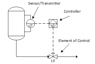
After defining the control strategy, it must be determined how to best implement this control strategy or logic in the process for efficient operation. Implementation of a control strategy is referred to as a control loop (shown in Figure 3), and relies on four fundamental elements working in a cycle:

1. The Process: Physical system to monitor and control.
2. The Sensor/Transmitter: Eyes of the control loop, measures the current state of the process variable and transmits that data.
3. The Controller: The brain. It receives measurement data from the sensor, compares the process variable value with the setpoint, calculates the difference error, and decides on a predictive/corrective action to take.
4. The Element of Control: The muscle. This is the physical device that directly changes the process based on the controller’s command, known as the manipulated variable. The most common and frequent element is a control valve, but it can also be a variable speed pump or an electric heater.

This control loop does not only turn things “on” or “off,” or does not simply set a control valve as fully open or fully closed (referred to as on/off or two-position control). On/off control is a legitimate strategy for appropriate applications (e.g., simple level cut-ins, pressure alarms, and temperature switches) but produces sustained cycling rather than stable setpoint tracking on processes with significant lag or dead time. To smoothly guide the process variable to the setpoint, the control loop instead uses a dedicated algorithm designed for a specific application called Proportional-Integral-Derivative (PID) control.

Type of Control Loops

Consider the level control loop depicted in Figure 3 in which dashed lines represent the signals passed between the control loop elements. A level-measurement device senses the level and sends a signal to the controller. The controller then compares the vessel liquid height with the desired setpoint and sends a controller output to the final element of control – in this case a control valve – which changes the valve position and therefore the flow that is allowed to pass through the valve. This response is generated by the proportional (P) algorithm described below.

Proportional Control (P)

Proportional Control is a type of feedback control algorithm where the controller’s output is directly proportional to the current error. The error is the difference between the setpoint and the actual condition of the process variable. The major limitation of this type of control is that it will not completely eliminate the error on its own. This remaining error is referred to as offset. The proportional controller calculates its output using the following linear equation:

Where,

• = output signal sent to the final control element
• = proportional gain (tuning parameter)
• = current error at time t, calculated as setpoint minus current process variable
• = bias (or manual reset) as the baseline controller output when the error is exactly zero, thus ensuring a valve does not just fully close in the moment the setpoint is briefly reached

Proportional-Integral Control (PI)

To avoid offset, integral control is added. This integral involves adding a term where the controller output is proportional to the integral of the error, in addition to the term that is proportional to the error. This is known as Proportional-Integral (PI) control. If there continues to be an error signal to the controller, the controller output (process input) will continue to change. Therefore, the integral of the error forces the error signal to zero. This type of controller implicitly accounts for the past (or history) system response.

The PI controller is defined as follows:

Where,

• = controller output at time t (e.g., the signal sent to the control valve)
• = current error between setpoint and process variable
• = proportional gain that determines how quickly the controller reacts to the current error
• = integral time, or fraction of the past time integrated to the response

This type of controller is known to commonly experience the following challenges:

• Oscillation: Because the integral term acts on past data, it inherently introduces a delay in the control response. In process control, this delay (also known as dead time) is the absolute time difference between the moment a controller makes a physical adjustment and the moment that adjustment first produces a detectable change in the process. If the integral gain is set too high (i.e., the controller acts too aggressively on accumulated error), the process will exceed the setpoint and begin to oscillate.
• Integral windup: If the controller’s output finds a physical limitation in the final element of control (e.g., control valve, speed variator, etc.) but the setpoint is reached, then the error remains. The integral term of the equation will continue to accumulate this error (windup), and the control loop will diverge instead of converging. When the process variable finally crosses the setpoint, the controller cannot immediately close or open the valve because it must first “unwind” that mathematical accumulation of error.

Proportional-Integral-Derivative Control (PID)

The next level of control complexity eliminates oscillation and integral windup with the addition of a term that accounts for the current rate of change (derivative) of the error. Using this term allows the controller to predict where the future error is heading and compensate for it. Generally, there are two ways to implement PID control: parallel and series.

The primary difference between a parallel PID and a series PID is in mathematical architecture, specifically where the integral and derivative terms either operate independently or multiply together and interact. For example, translating tuning parameters from dynamic process models to a live Distributed Control System (DCS) requires strict verification of architectural compatibility. Applying parallel-optimized parameters directly to a series-based controller without appropriate mathematical translation will significantly alter the control loop’s dynamic response, carrying a high risk of loop destabilization.

In a parallel PID architecture, the proportional, integral, and derivative actions are calculated independently based on the error, and their results are simply summed together. The parallel PID equation is as follows:

Where,

• = transfer output of controller

• = proportional gain tuning parameter

• = integral time

• = derivative time

• = first-order filter (; where is typically 0.1)

Two key characteristics of parallel architecture are the lack of interaction between integral and derivative terms and the intuitive tuning of both variables. If for some reason the process requires frequent setpoint changes, implementing this architecture may not be desirable. A step setpoint change, for example, would cause the derivative of the error to be infinite and a spike in the manipulated variable; this behavior is known as derivative-kick. For this reason, the derivative action is often based on the process output rather than the error.

In a series PID architecture, the PI term and the proportional-derivative (PD) term are multiplied together. This means the output of one term feeds into the other, as shown in the following equation:

Series architecture key characteristics include the interaction between the integral and derivative terms increasing the actual proportional gain applied to the system and the addition of tuning complexity as if the derivative time (term) is increased to damp an overshoot. This causes the proportional gain to increase, too, which might cause oscillations.

The following table compares the two types of architecture:

Feature	Parallel	Series
Term Interaction	None, I and D are independent	High, D interacts with P and I
Mathematical Structure	Additive (P + I + D)	Multiplicative [(P + I) x (P + D)]
Effective Gain	Equals the entered	Higher than entered (multiplied by)
Primary Use Case	Modern DCS defaults, academic theory, algorithmic tuning	Legacy system retrofits, analog hardware emulation
Tuning Difficulty	Straightforward	Complex if heavy derivative action is required

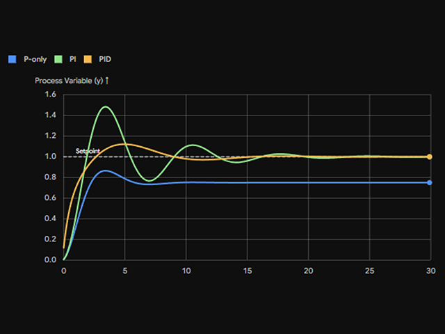
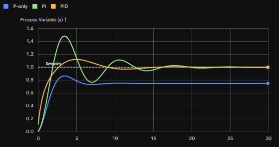
For further comparison, the following graph shows the behavior of the three different controllers. Notice the proportional control curve reacts quickly but flatlines below the setpoint (offset); the PI control curve reaches the setpoint, but overshoots and oscillates before settling; and the PID control curve (with the addition of the derivative term) dampens the overshoot and settles smoothly.

Instrumentation

Instrumentation is critical to the control loop’s ability to work efficiently. The most important pieces of instrumentation are a sensor (measurement device), controller (brain of the control system), and actuator (device to carry out the control action from the PID controller). The sensor will measure the process variable, and based on the sensor signal, the controller will determine how much to vary the actuator, which will adjust the process variable by changing the manipulated input/variable to the system.

There are many common sensors – including temperature, level, pressure, flow, composition, and pH – used for chemical processes. The most common manipulated input is the valve actuator signal, but speed variators and modular switches can be included as final elements of control.

Each device in a control loop must supply or receive a signal from another device. When these signals are continuous, such as electrical current or voltage, they are analog. If the signals are communicated at discrete intervals of time, they are digital.

A common analog measurement device might supply either a 4- to 20-mA or 0- to 5-V signal as a function of time. Pneumatic analog controllers use instrument air, as well as a bellows-and-springs arrangement, to calculate a controller output based on an input from a measurement device. The controller output of 3 to 15 psig is sent to an actuator, which is typically a control valve where the pneumatic signal moves the valve stem. New electronic analog controllers receive the same amount of signal current or voltage from a measurement device and use an electronic circuit to determine the controller output.

Currently, most devices and controllers are based on digital communication technology. A sensor may send a digital signal to a controller, which then does a discrete computation and sends a digital output to the actuator. Very often, the actuator is a valve, so there is usually a digital-to-electronic analog converter involved. If the position of the valve stem is modified by a pneumatic rather than electronic actuator, then a current-to-pneumatic analog converter may also be used. Digital control system design techniques explicitly account for the discrete (rather than continuous) nature of the control computations. If small sample times are used, the tuning and performance of the digital controllers are nearly equal to that of analog controllers. Selecting the right communication protocol is an important part of instrument specification, since the choice directly affects loop performance and plant safety. Common digital and hybrid communication protocols in industrial process plants include Highway Addressable Remote Transducer (HART), which superimposes a digital signal on the conventional 4-20 mA loop); FOUNDATION Fieldbus (H1 and HSE); Profibus PA/DP; and EtherNet/IP. The selection of communication architecture affects loop scan rate, intrinsic safety zoning, power distribution, and DCS integration. These distinctions are relevant to control loop design and instrument specification and should be addressed in any complete treatment of instrumentation for process control. The distillation column reflux controller example below illustrates several of these instrumentation and control principles applied to a real process.

Application Example – Distillation Column Reflux Controller

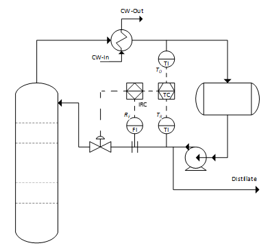
One common controller included in the distillation column control scheme is the internal reflux controller. This control loop implementation has a major strength in its ability to minimize the impact of disturbances in the cooling medium on the distillation column. This controller automatically adjusts the reflux flow rate for changes in reflux subcooling duty.

Upon entry into a column, a subcooled reflux quickly heats up to its boiling point by condensing the overhead vapor. The liquid in the top section therefore equals the external reflux plus that condensate. Frequently, the condensate makes up about 10 to 30% of the internal reflux flow rate, and it is not uncommon to find situations where it exceeds 40% of the internal reflux. Subcooling variations alter the quantity of condensate formed and are therefore reflected in changes in the reflux rate. The function of the internal reflux controller (IRC) is to compute the column internal reflux and control it at the desired setpoint. A simple and approximate correlation used is:

Where,

• = external reflux

• = internal reflux

• = overhead reflux temperature

• = subcooled reflux temperature

• = ratio of the liquid heat capacity divided by the latent heat

, , and are measured, and is calculated with the above equation. This calculation is performed by the IRC instrument.

Consider a sudden increase in subcooling. will drop and raise . The IRC will close the reflux control valve to bring to its set value. External reflux flow rate will be reduced, but the column will see no change because the IRC will maintain the internal reflux stable. The logic of the IRC is to regulate the reflux flow rate by cascade-controlling the reflux temperature. In this cascade control, multiple output measurements (temperatures , measured before the accumulator; and , measured after it) are used to improve the response of the most important and primary output (control valve opening percentage) to a disturbance (condenser duty or cooling water flow rate). The following figure shows how a general distillation column reflux control loop is implemented.

Conclusion

Well-designed control loops are the backbone of safe, efficient, and profitable process operations, but getting them right requires disciplined attention at every stage, from strategy definition through instrumentation selection and final tuning. As this article shows, even well-understood tools like PID control carry real implementation risks when architecture, protocol, or application details are overlooked. Equity Engineering’s Process, Automation, Controls, & Electrical (PACE) team helps clients navigate exactly these challenges, from control strategy development and loop tuning to instrumentation reliability and DCS integration, ensuring control systems perform as designed under real operating conditions.

References

• Smith, C. A., Corripio, A. B. Principles and Practices of Automatic Process Control, John Wiley & Sons, Inc., 3^rd edition, 2005.
• Luyben, M. L., W. L. Luyben. Essentials of Process Control, McGraw-Hill, 1997.
• Luyben, W. L. Process Modeling Simulation and Control for Chemical Engineers, McGraw-Hill, 2^nd edition, 1999.
• Luyben, W. L. Distillation Design and Control Using Aspen Simulation, McGraw-Hill, 2^nd edition, 2013.
• Routh, E. J. Dynamics of a System of Rigid Bodies, Part II., Macmillan, 1995.
• Skogestad, S. “Simple Analytic Rules for Model Reduction and PID Controller Tuning,” Journal of Process Control., Vol. 13, 219-309.
• Symmetry Process Simulation Platform User’s Manual, 2026.
• Control Tutorials for Matlab® & Simulink®, PID Controller Design, 2026.
• Shinskey, F. G. Distillation Control, McGraw-Hill, 2^nd edition, 1984.