Due to the cyclic operation of Reformer Unit reactors, fatigue is often a damage mechanism of concern not only of the reactors themselves, but also for other assets supporting the reactors such as piping and valves. This case study investigates fatigue cracking of Motor Operated Valves (MOVs) that cycle flow into and out of the reactors to support decision-making regarding inspection and repair planning of the valves.
Historically, a client’s inspection identified surface crack-like flaws on the ID bore of a number of MOVs. During their most recent turnaround, the client discovered similar cracking in three (3) of the Class 400 MOVs in their Catalytic Reforming unit (Figure 1), the most severe being 0.150 inches (3.81 mm) deep and 1.75 inches (4.45 cm) long in a section of the MOV body that is 1.58 inches (4 cm) thick. Since only three (3) of the 33 valves have been opened, the client was concerned with the presence of cracks in additional valves, how the level of cracking could be managed, and whether repairs were required. Thus, E2G was contracted to provide guidance on acceptable flaw sizes to assist the client in making decisions on MOV repairs during the upcoming turnaround.

The Root Cause of Cracking
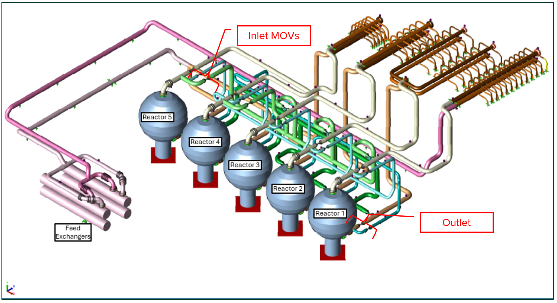
The Reformer Unit under investigation consists of five (5) reactors: four (4) reactors in process operation and one (1) in either regen or standby operation; see the Reformer Unit layout shown in Figure 2. Each reactor has three (3) inlet and outlet MOVs. A typical regen operation lasts about 30 hours, and all five reactors are regened in about seven (7) days, with the last regen swing reactor remaining in standby for about 23 days. The 23 days of standby results in cooling of the process/regen gas entrapped in the deadlegs close to ambient temperatures. The cyclic operation of the MOVs was noted to range from 10 to 14 cycles/yr. For the Reformer Unit under investigation, the valve sequencing is such that the maximum length of the deadlegs could be as high as 100 feet (30.5 m). When the reactor in standby is ready to be brought back into process, the MOVs experience a thermal shock caused by cold process deadleg media passing through the MOVs, followed by hot process media. Such frequent thermal shock events are believed to be the cause of cracking on the ID bore of the MOVs.
MOV Geometry
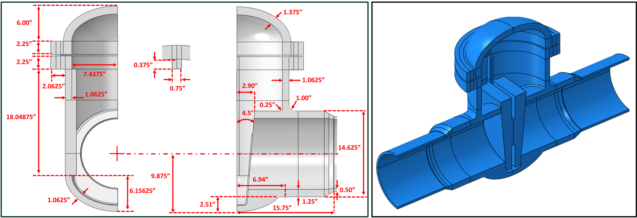
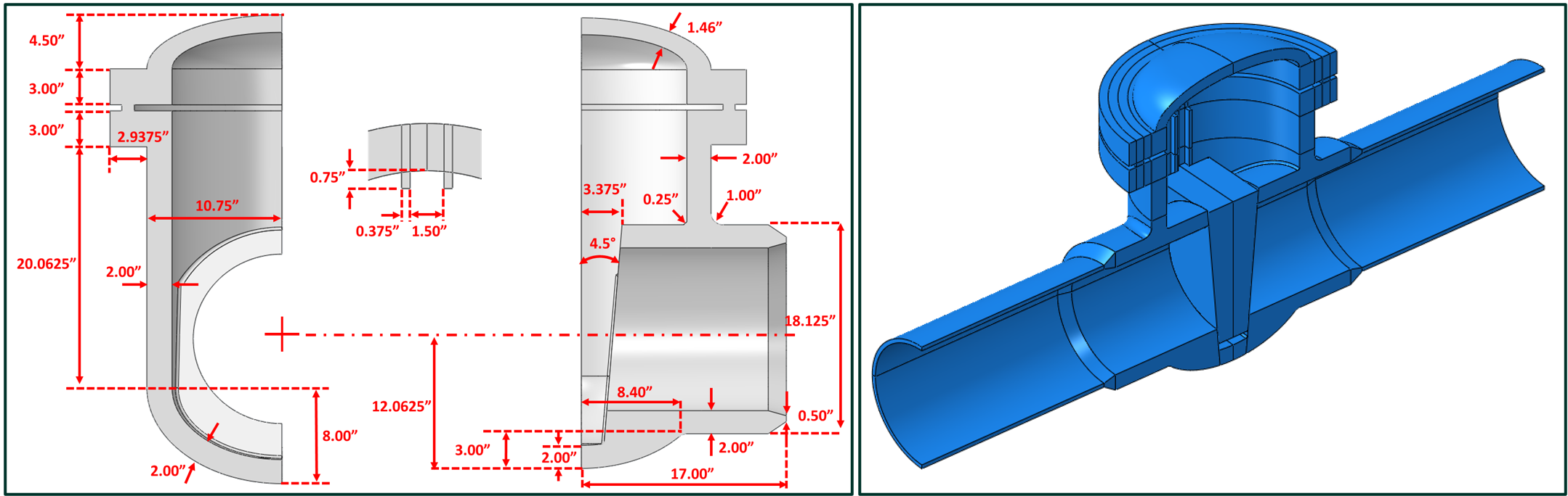
Prior to performing any computational fluid dynamics (CFD) analysis or finite element analysis (FEA), the geometry of the MOVs being assessed must be modeled. For this project, both NPS 12 and NPS 16 Class 400 MOVs were chosen. These are both rising stem buttwelded gate valves utilizing a flex wedge for the NPS 12 MOV and a split wedge for the NPS 16 MOV. Insulation was removed from two valves and field dimensions were obtained of the actual valve bodies. Because the unit was in operation, however, internal access was not possible. Therefore, E2G utilized valve internal dimensions obtained from two prior MOV assessments (same size valves) where sacrificial MOVs were cut into quadrants and detailed internal dimensions determined. The final dimensions used for the finite element model (FEM) and the resulting model geometry are shown in Figure 3 and Figure 4 for the NPS 12 and NPS 16 MOVs, respectively.
Computational Fluid Dynamics Analysis
The thermal shock caused by cold deadleg passing through the valves followed by hot process that occurred when the valves were opened after a long standby was simulated using CFD analysis.
1. Steady-State CFD Model
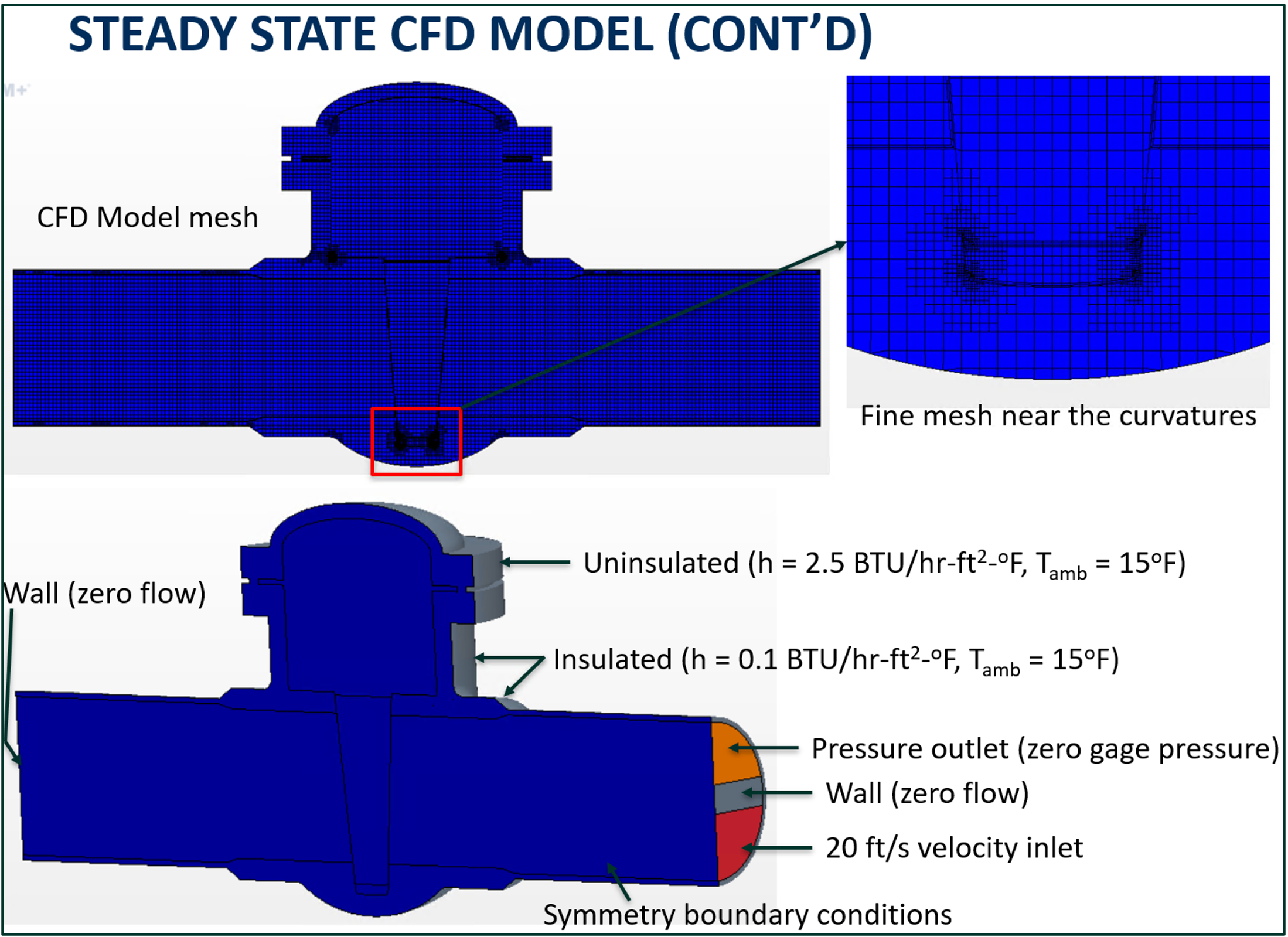
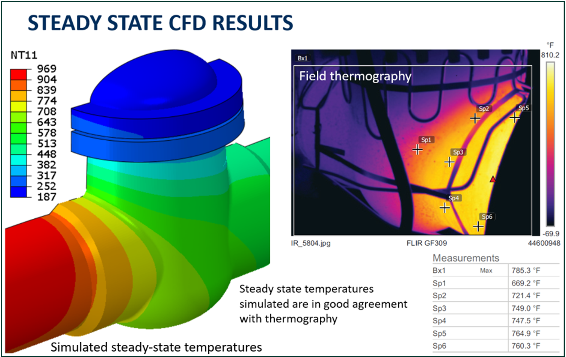
Initially, the three dimensional (3D) solid models of the representative MOVs were developed in a commercial finite element software, Abaqus. The models were then imported into a commercial CFD software, Star-CCM+. The standby reactor MOVs that are located closer (3 to 4 feet / 91 to 121 cm) to the process flow of the other reactors stay warm even when they are closed. The process fluid recirculates in the 3 to 4 feet (91 to 121 cm) of deadleg and keeps the MOVs warm. To approximate the effect of the re-circulating process fluid in the 3 to 4 feet (91 to 121 cm) of deadleg, one end of the pipe was divided into three sections: top, mid, and bottom (Figure 5). Velocity inlet boundary conditions with a velocity magnitude of 20 ft/s (6m/s) were defined on the bottom section. Temperature of the fluid was chosen based on the temperature screenshots provided by the client to represent the process conditions just before the valves opening. Convective heat transfer boundary conditions were applied on the outer surfaces of the valve and the bonnet body. The effect of insulation on the pipe and the valve body was included in the calculation of heat transfer coefficients. The chosen modeling assumptions seemed to capture the steady state temperatures reasonably well. See Figure 6 for comparison of field thermography and the estimated temperatures from the CFD model. Steady-state temperatures were extracted from the CFD model and mapped as initial temperature conditions in transient simulations.
2. Estimation of Deadleg Temperatures
Whenever a reactor is in standby, process/regen gas gets entrapped in the deadlegs and cools down with time, potentially reaching ambient temperatures. However, the ends of the deadlegs stay warm due to their proximity to the process fluids flowing through the opened MOVs. The deadlegs were not modeled explicitly in the CFD analysis. Rather, closed-form fin calculations were performed to estimate the temperature distributions in the deadlegs.
3. Inlet Transients
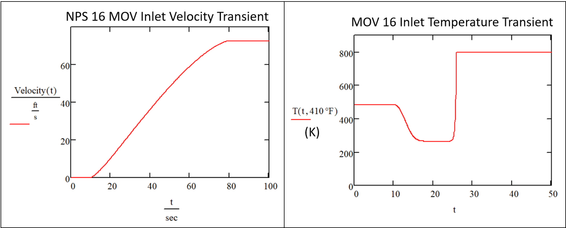
The estimated deadleg temperatures were assigned as inlet temperature transients in the CFD model. The volume flow rate at the inlet was assumed to scale with percent area opening of the gate. The percent area opening was estimated by subtracting intersected cross-sectional area between the two circles (vessel ID and gate OD). The rate of temperature change in the temperature transient was estimated using the volume flow rates. The fin calculations were performed by assigning average steady-state temperatures from the CFD models as the base temperature. The fluid flowing to the deadleg was assumed to be at the maximum operating temperature. The estimated inlet velocity and temperature transients for one MOV are shown in Figure 7.
4. Transient CFD-FEA Co-Simulation
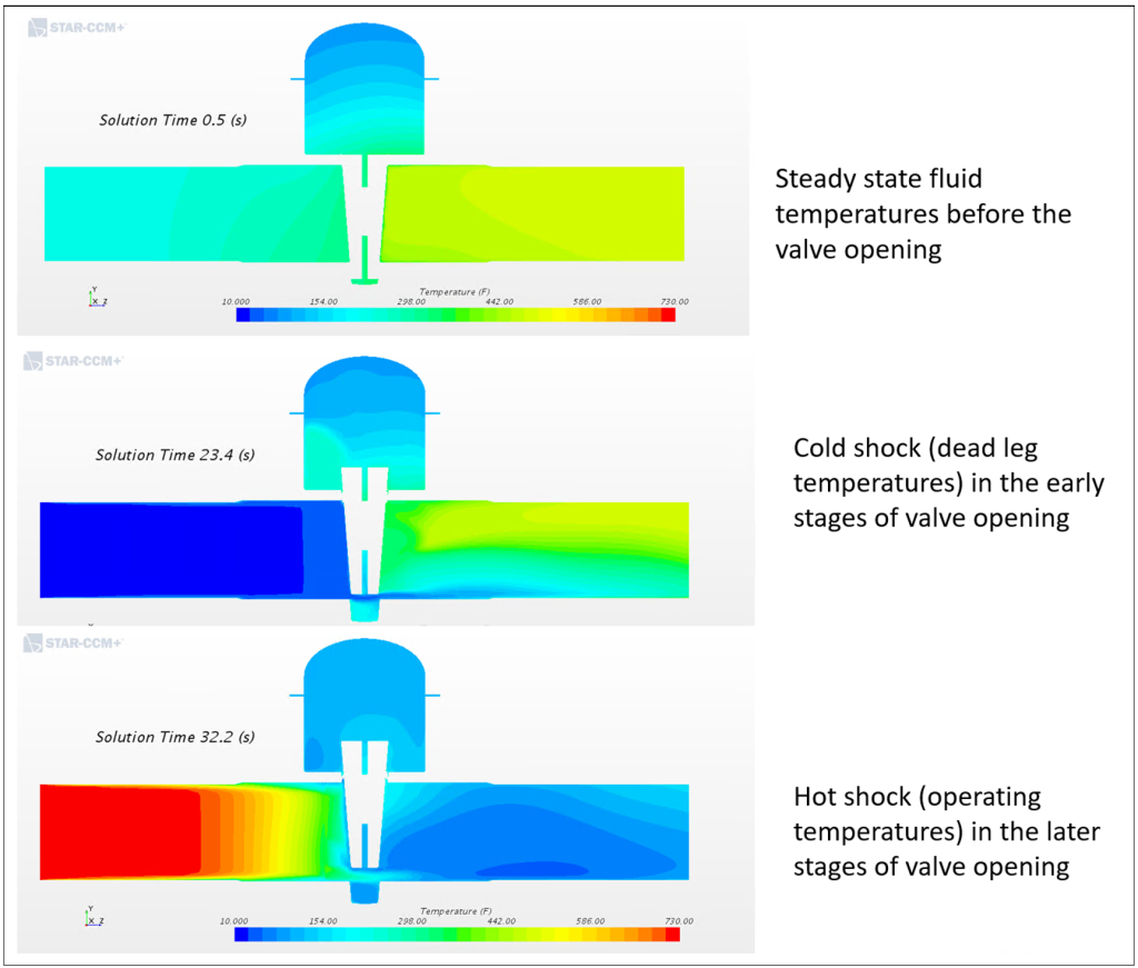
Transient CFD-FEA co-simulations were performed to determine temperature distributions in the valve body during the valve opening transients. Valve body solid domain is modeled in FEA software Abaqus whereas the fluid domain is modeled in CFD software Star-CCM+. For the solid domain, the initial temperatures were mapped from steady-state CFD model. Heat transfer coefficients on the OD surfaces of the valve body were similar to steady state CFD model (Figure 5). On the ID of the solid domain, heat fluxes were mapped from the CFD model. For the fluid domain, the inlet velocity and temperature transients were as per shown in Figure 7. Overset mesh with zero gap was defined for the valves. The client-specified MOV opening times were simulated in the CFD to properly capture the transient effects. Interface temperatures for the fluid domain were imported to the Abaqus FEA model. Both the Abaqus and Star-CCM+ were run simultaneously. The resulting FEA output database files were then used for thermal stress analysis as described in the following section of this article. A CFD plot of the thermal distribution for one of the MOVs upon gate opening is shown in Figure 8.
Finite Element Analysis
An FEM of the valve body and a portion of the attached piping was constructed using 3D solid elements. Half symmetry was assumed to reduce the model size. Loading incorporated into the model included internal pressure loading and the actuator loading on the valve gate. Contact between the valve gate and valve body is explicitly simulated in the model. An overview of the FEA model is presented in Figure 9.
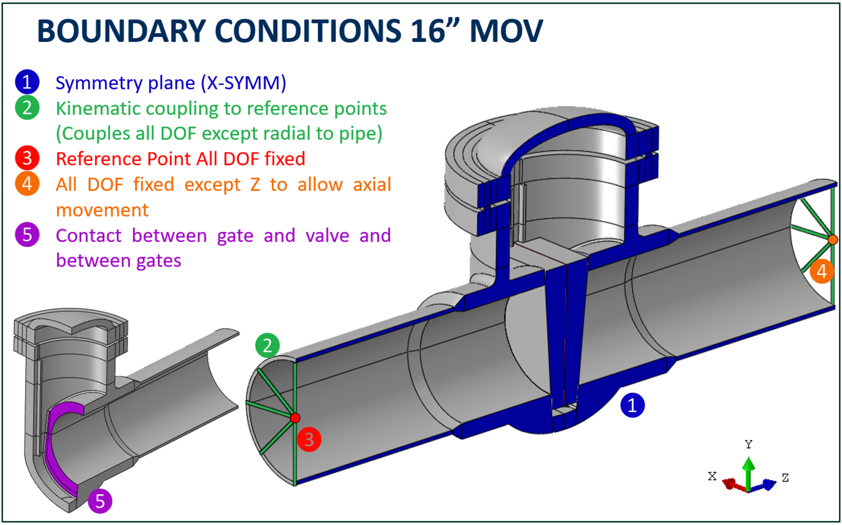
To simulate the thermal transient computed in the CFD model, the transient thermal distributions were directly imported into the FEM. For a point in time, the FEA computed the thermo-mechanical stress state for both the thermal stress (caused by the imported nodal temperature distribution from CFD) and the mechanical stress (caused by pressure and [when applicable] gate loading). A plot of the elastic stresses due to mechanical loads as well as thermal loads is presented in Figure 10.
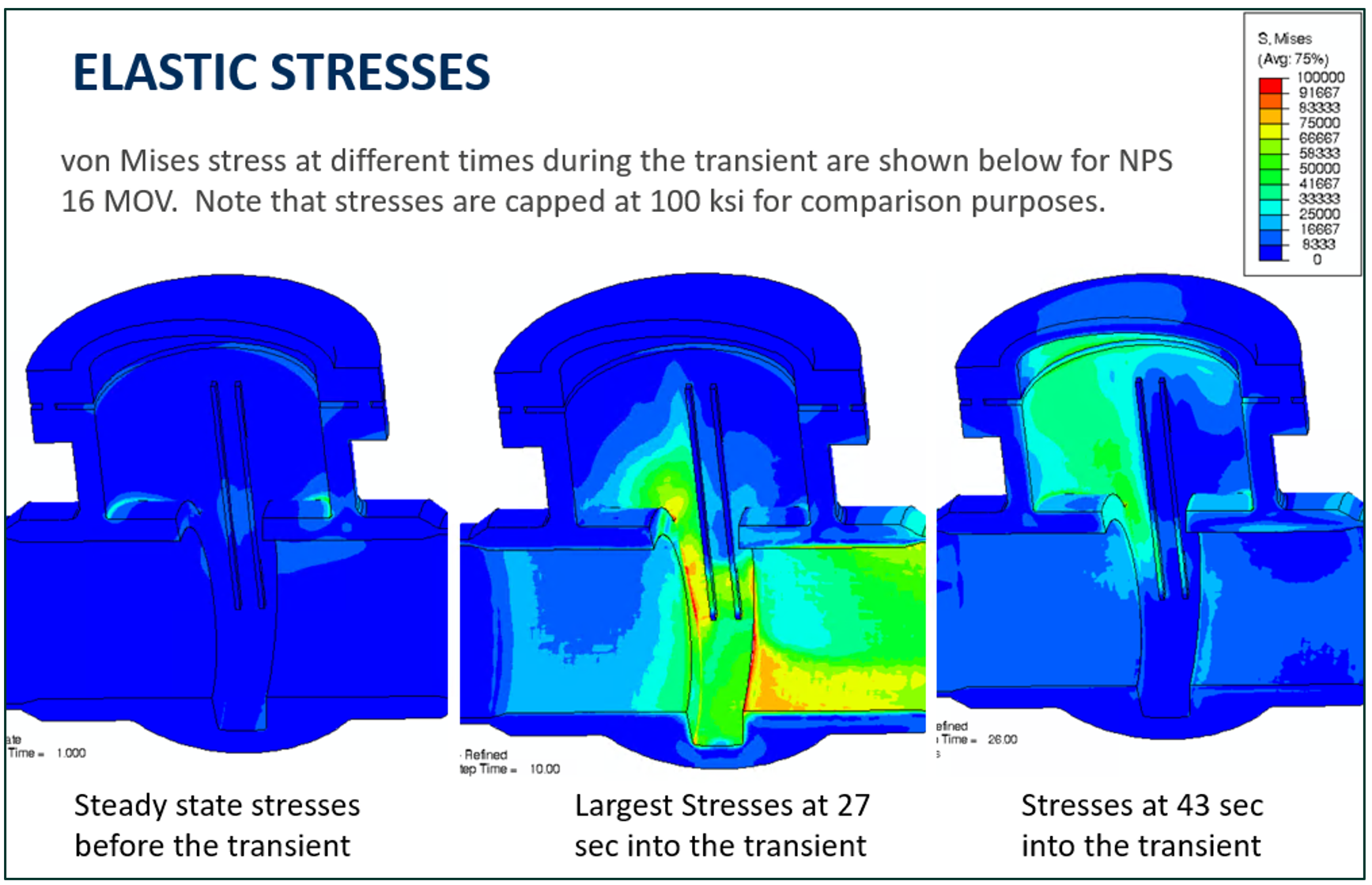
In addition to the elastic stress analysis, 25 stress cycles were simulated using an elastic-plastic material model, which included kinematic hardening for the 1.25Cr-0.5Mo MOV material to predict the stabilized stress response of the valve body.
Fatigue Calculations
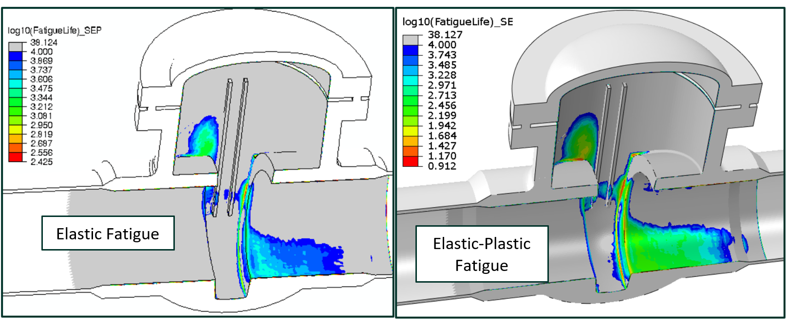
A fatigue assessment was performed to identify the critical hot spots on both MOVs where thermal-fatigue cracking is of most concern. The fatigue analysis was performed using both elastic stresses and the stabilized elastic-plastic response. A smooth bar fatigue evaluation in accordance with Part 14 of API 579 was used. In comparison, the elastic fatigue assessment produced more limiting fatigue damage when compared to the stabilized elastic-plastic fatigue evaluation; however, both fatigue methods consistently identified limiting locations. This is demonstrated by plotting the predicted fatigue life for both methods as shown in Figure 11. Note that the contour plots are in the units of log cycles where log cycles are defined as:
Where, N is the number of predicted fatigue cycles. The results of the fatigue assessment indicate fatigue prone locations consistent with the regions of cracking identified via inspection.
Crack Growth Calculations
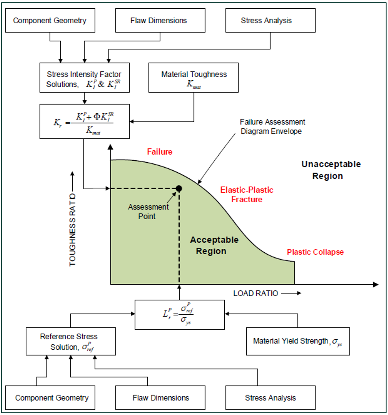
To further understand the progression of the identified cracking, crack growth calculations were performed in accordance with Part 9 of API 579 utilizing through-wall stress distributions obtained from the FEA. To perform the fracture mechanics calculations, determination of the limiting flaw size is required. The procedure to evaluate crack-like flaws is based on the failure assessment diagram (FAD) method in accordance with API 579. In a FAD assessment, results from the stress analysis, material strength, and fracture toughness are combined to calculate a toughness ratio and load ratio. These two quantities represent the coordinates of a point that is plotted on the FAD to determine acceptability. The diagram presented in Figure 12 provides an overview of the FAD assessment methodology.
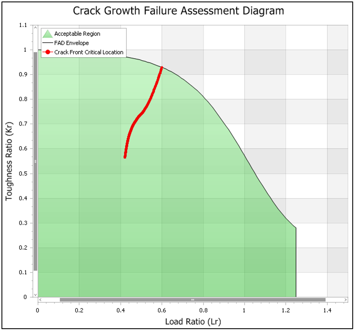
Crack growth calculations were performed by cycling from the transient stress-state with the largest ID tensile stress to the stress-state with the largest OD tensile stress. Initial flaw size was iterated upon to determine an initial flaw size (20:1 length-to-depth ratio) that would growth to the critical flaw depth in 1,000 cycles (40 years at 25 cycles/year). The cyclic rate of 25 cycles/year was conservatively chosen for the crack growth calculations to provide roughly a margin of 2X on the typical operation of 10 to 14 cycles/year. This initial flaw size could then be used by the client to identify cracks requiring repair. The plot presented in Figure 13 shows crack growth behavior in reference to the FAD as defined in API 579 for an example case. Failure occurs when the crack front reaches the edge of the FAD curve.
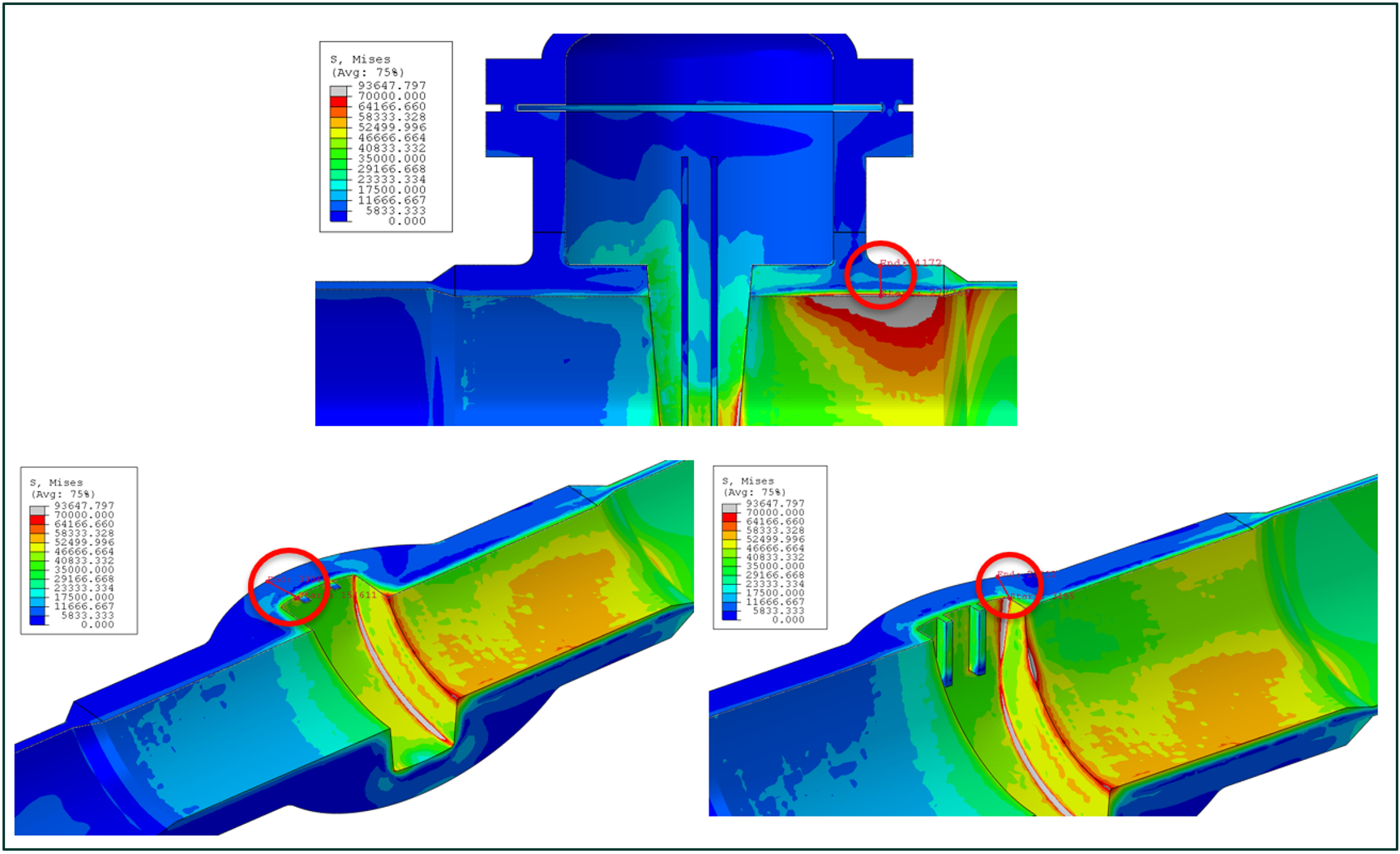
Limiting locations assessed via crack growth calculations are presented in Figure 14. Iterating on flaw size until the cracking growth calculations produce an unstable flaw in 1,000 cycles resulted in a limiting flaw depth of (0.350 inches/8.89 mm, limited by stresses at the gate guide). The client can use this resulting flaw size to guide inspection and make run/repair/replace decisions when future cracking is identified in the valves.
Summary
In this case study, a root cause of MOV cracking was verified by simulating the thermal shock caused by cold deadleg followed by hot process passing through the MOVs. The critical MOVs (location of those with large deadlegs) and regions within the MOVs that this analysis predicted to have the highest risk of fatigue damage aligned with field-observed crack locations. Acceptable flaw depths were provided to ensure a flaw does not go unstable within 1,000 cycles (40 years at 25 cycles/year), which can be used to make a decision regarding repair. Ranking of the MOVs based on their deadleg lengths was provided to guide future inspection and potential valve replacements. The IR study provided by the client also aligned with the FEA thermal simulations, which indicated the MOV bodies stay very warm with or without the steam tracing in operation. Thus, the client may consider removal of existing stream tracing because the MOV body temperatures are maintained above 300°F (148◦C), which sets the valve body toughness at the upper shelf.
Please submit the form below with any questions for the authors: