Introduction
Refractory linings are commonly used to protect pressure vessels and piping components from hot process conditions and minimize heat losses in the oil & gas and petrochemical industries. Refractory linings can deteriorate in service due to loss of physical properties with length of service, spalling due to vibration or thermal cycling, improper design and installation, failures of refractory supports, etc. Refractory degradation can lead to eventual failure of the refractory, exposing the pressure vessels and piping components to temperatures significantly above the design temperatures, resulting in hotspots. The components with hotspots are prone to excessive creep damage and potential creep-fatigue damage if in cyclic service, especially at the edges of the hotspots because of higher thermal gradients and stresses. Further degradation may occur due to oxidation corrosion at elevated temperatures or other material-specific damage mechanism. For example, materials such as carbon steels may be subjected to graphitization over time operating at temperatures above 800°F (426ºC) if hotspots are not addressed in a timely manner.
Managing Refractory Degradation with Inspections
A periodic infrared (IR) inspection program is recommended to monitor for any hotspots/refractory degradation in refractory-lined equipment. If hotspots are noticed, the root cause of the refractory degradation should be investigated, and remedial measures should be taken before the hotspots’ temperatures exceed the design temperature. If periodic IR inspections are not possible, temperature-sensitive paints can also be used as an effective indicator of hotspots/refractory degradation. Additionally, the nature of oxidation scale and/or paint condition in one area versus the neighboring areas can also be an indicator of hotspots/refractory degradation.
As a short-term measure, steam/air cooling can be applied to the affected areas to bring down the hotspot temperatures below the design temperatures. However, it should be noted that steam/air cooling may not be effective at reducing the temperature through-thickness for thick-walled components and is not practical if the hotpots are larger in size. Additionally, IR inspections are not accurate when the steam cooling is being applied, which makes it difficult to monitor the hotspot temperatures. Installation of skin thermocouples (if practical) may alleviate this issue, but again with thicker-walled components, the surface temperature may not be indicative of through-wall temperature gradients.
After the root cause of the refractory degradation is fixed, it is recommended to inspect the affected areas for any distortion or cracking. Additionally, an advanced engineering analysis is recommended to determine the impact of the hotspots on the integrity of the equipment. This is recommended even in cases where refractory repair is completed and inspection is performed, as permanent material damage due to creep and/or creep-fatigue may not be evident with typical inspection. A case study of such analysis is discussed next.
Advanced Engineering Analysis to Determine the Impact of the Hotspots on Integrity of the Equipment
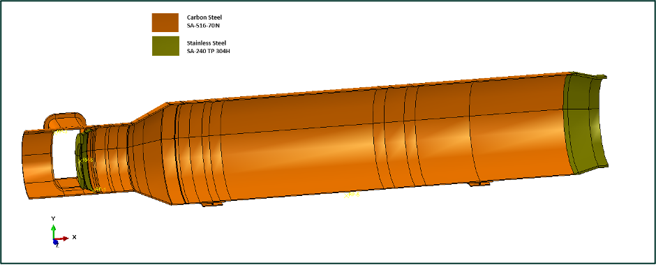
Consider the case of a slide valve and downstream expansion region which was originally designed to “cold wall” conditions for the bulk of the pressure boundary (cold wall implying outside the creep temperature boundary) (Figure 1 – Top). All the carbon steel regions in Figure 2 were designed to a maximum of 650°F (343ºC) at 53 psig internal pressure. The original design was conducted with reference to ASME Section VIII Division 2 Part 5.
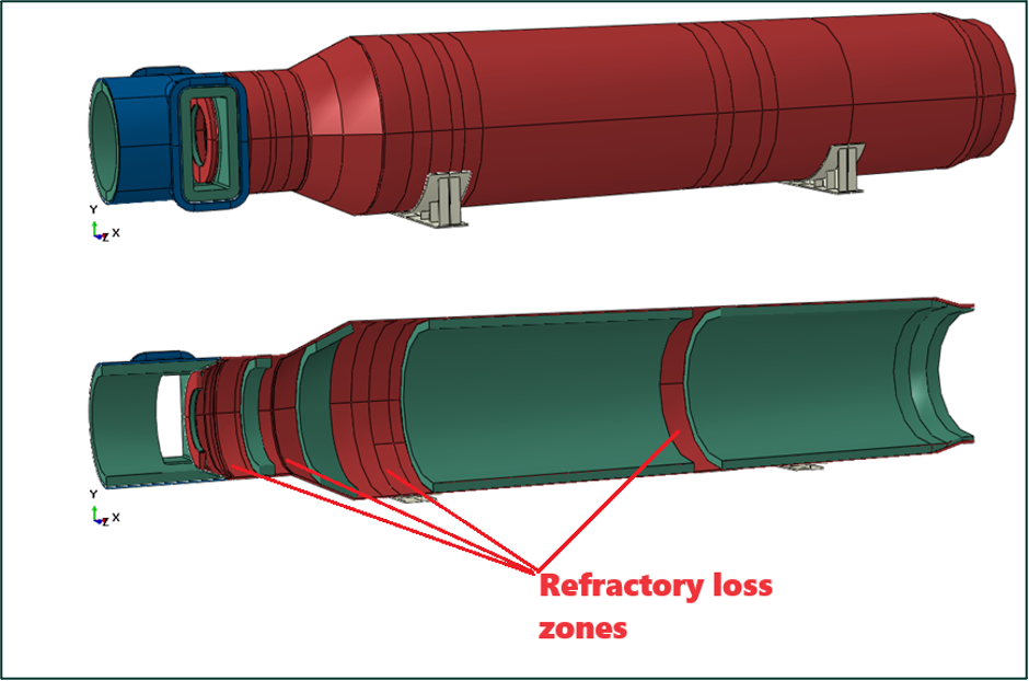
An alteration to the internal refractory lining resulted in significant degradation to 4 circumferential “rings” of the refractory lining of the component (Figure 1 – Bottom). In turn, the refractory damaged regions began to experience wall temperatures in excess of the design conditions – up to 890°F (426ºC). The equipment owner was able to control the wall temperatures using external air cooling; however, since the creep transition temperature for SA-516-70N carbon steel is approximately 750°F (399ºC), there was significant concern regarding continued use of the slide valve (notwithstanding, 890°F (426ºC) is 240°F (115ºC) higher than the original design cold wall condition of 650°F (343ºC)).
E2G was contacted to assess the fitness for service of the slide valve piping section with 4 circumferential hotspot regions set to a maximum wall temperature of 1000°F (538ºC) for a duration of 5 years. (1000°F was chosen to give the current cooling efforts reasonable headroom for future progression of the refractory degradation.) A Level 3 fitness-for-service analysis incorporating creep was proposed. The analysis was conducted as per the guidelines of API 579 and ASME Section VIII Division 2 Part 5 wherein the standard failure modes of plastic collapse, local failure, ratcheting, buckling, fatigue, and (in this case) the supplementary failure modes of creep rupture and creep-fatigue are considered. This article will focus on the creep-fatigue failure mode.
Creep Analysis
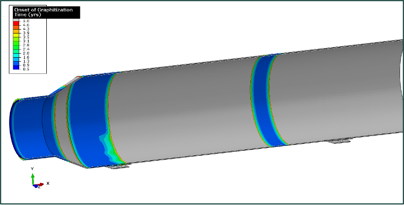
Typically, carbon steels such as SA-516-70N are not operated at temperatures above 750°F (399ºC) for extended periods of time due to their relatively poor performance in creep conditions. Since the objective of the fitness-for-service analysis was to determine the feasibility of operating with a maximum external wall temperature of 1000°F (538ºC) until 2029 (where a turnaround will address the refractory deficiencies), the SA-516-70N carbon steel is likely to experience graphitization. An estimate of the graphitization initiation time is shown in Figure 4. The estimate is based on the following relation (Foulds & Viswanathan, 2000):

Where T is the nodal temperature of a point in the model. Since all the hotspot regions will experience some graphitization before end of year 2029 and may have accumulated some from prior operation, all the materials were given minimum creep properties with Δsr= -0.5 and Δcd= +0.3. This shift effectively moves the material to lower-bound creep properties. API 579 provides graphitized carbon steel Omega and strain rate coefficients, and the intent of these graphitized properties is to employ a Δsr= -0.5 adjustment to the base carbon steel initial strain rate (A0) coefficient. The Δcd= +0.3 shift on the Omega parameter was applied as a further conservative shift to lower-bound properties given the severe service.
E2G’s proprietary Omega creep software was utilized for this assessment. The Omega creep software used by E2G is a user subroutine that incorporates an extended form of the Materials Properties Council (MPC) Omega creep model into an Abaqus finite element analysis (FEA) model. In this model, the creep strain rate, Ėcr , increases from its undamaged value, Ė0, as creep damage, D, accumulates at a damage rate, Ḋ, that depends on the uniaxial omega parameter, Ω, according to equations 10.30 through 10.42 in API 579 Part 10. The user subroutine affords the capability to plot the cumulative creep damage in a component subjected to temperature conditions inside the creep envelope of a given material.
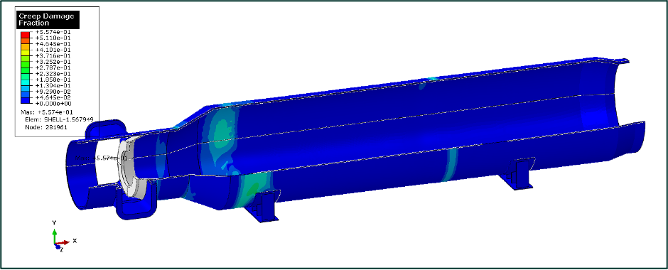
The creep damage accumulated in the intended operational window prior to repair was determined through direct simulation of the complete future timeline. The accumulated creep damage results (56% maximum) are shown in Figure 5.
Fatigue Analysis
The temperature and pressure cycles for the slide valve are out of phase. In order to find closed hysteresis loops, a rainflow (or other) cycle counting procedure must operate directly on the stress (or strain) to define the number of unique (and significant) cycle ranges in a given time history. To this end, a transient coupled thermo-mechanical analysis was performed using the start-up/shutdown data directly for a typical year of operation, and the Mises stress from hotspot locations were extracted and run through a rainflow counting procedure. For each closed stress hysteresis loop (k), an elastic fatigue analysis where the thermal stress is not partitioned from the total stress was conducted. The equivalent alternating stress amplitude was computed as:
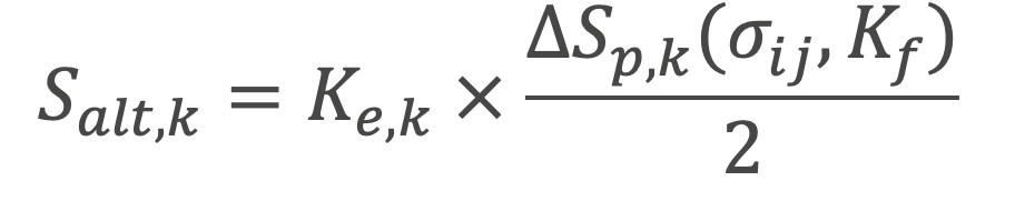
Where Ke,k is the fatigue penalty factor for a given region in a given component on the kth cyclic stress range, and ΔSp,k(σij,Kf) is the raw equivalent alternating stress range which is a function of the stress tensor components σij and (if applicable) a geometry-based weld fatigue penalty factor Kf. Typically, Ke,k is calculated by linearizing through-wall stresses within a given region and comparing the local primary membrane plus bending plus secondary stress to three bins (equations 14.25-27 of API 579 Part 14). This methodology can be inefficient for large models and, as such, the alternative methodology for calculating Ke,k described in API 579 Part 14.4.3.2.4 is used. In this method, Ke,k is defined by the following:
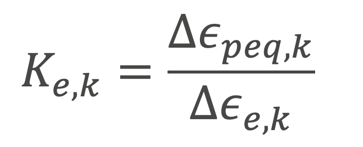
Where ΔEpeq,k is the equivalent plastic strain range for the kth cycle and ΔEe,k is the equivalent elastic strain range for the same cycle defined in equations 14.38 and 14.39 of API 579 Part 14, respectively. This definition facilitates the implementation of a Ke,k field directly as an output in Abaqus. In this component, the main pressure boundary welds are of quality Level 1 (API 579 Part 14 Table 14.6) and are assumed to be left in the as-welded condition with only minor grinding; thus, the weld regions of the model will receive a stress amplitude penalty factor of Kf = 1.2.
The ASME Smooth Bar Method outlined in Part 14 paragraph 14.4.3.2 of API 579 was used to evaluate the maximum number of permissible cycles for each cycle range. Since the entire pressure boundary under the scope of the fitness-for-service analysis is comprised of SA-516-70N carbon steel, only curve 14.B.1 is used. It is typically preferred to utilize the Structural Stress Method for welded locations in lieu of the Smooth Bar Method with weld-specific penalty factors; however, this method requires stress linearization at all welded locations of interest, which is very time-consuming for an analysis of this scope and complexity. The Smooth Bar Method with penalty factors is generally taken to be a more conservative approach and, therefore, provides a suitable solution in this scenario where fatigue damage is required at all locations in the model.
The fatigue life was calculated for each cycle k (total number of cycles to failure, Ni), and the combined fatigue damage (Df) is calculated based on the number of cycles of each type k (ni) using the Palmgren-Miner cumulative damage model:
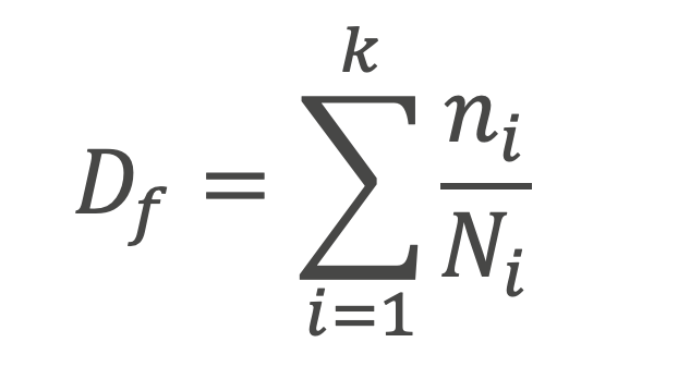
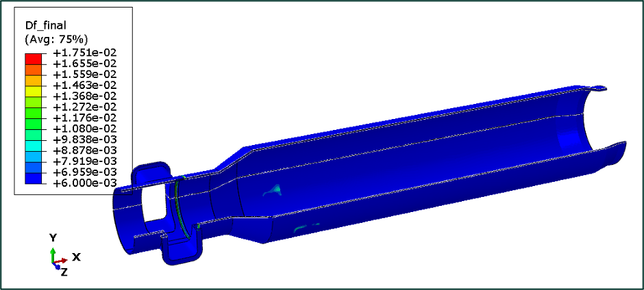
Similar to the creep simulation, the fatigue damage accumulated in the intended operational window prior to repair was determined through direct simulation of the complete future timeline. The accumulated fatigue damage results (1.8% maximum) are shown in Figure 6.
Creep-Fatigue Interaction
Creep-fatigue is evaluated based on the appropriate creep-fatigue interaction diagram for the material under consideration (Figure 7). The fatigue and creep damage metrics (Dc and Df , respectively) are supplied from independent creep and fatigue analyses and plotted as an evaluation point (D = (Df , Dc)) on the creep-fatigue interaction diagram. If the evaluation point lies on or below the allowable envelope, the component is considered acceptable for the operational history analyzed.
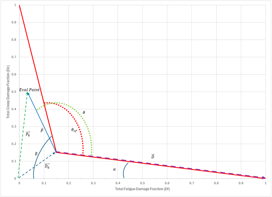
The creep-fatigue damage field results were computed by extracting the nodal creep damage and fatigue damage values and combining them into the creep fatigue damage metric θ (see Figure 7). If 360° ≥ θ ≥ (θcf = 110°), then the point lies within the allowable creep fatigue damage envelope and the component is acceptable. If 0° < θ < (θcf = 110°), then the point lies outside the creep fatigue damage envelope and the component is not acceptable. The creep fatigue damage metric used in this study provides a convenient way of assessing all the points in the FEA model for creep-fatigue acceptability using a single parameter.
For the slide valve under investigation, the calculated minimum and maximum theta values are 118.9 ≥ θ ≥ 180.0 (recall that the limits for compliance are 110 ≥ θ ≥ 360). The creep fatigue damage metric θ falls inside the compliance inequality for the entire component. Therefore, the component is considered suitably resistant to creep fatigue under the assumed hotspot conditions.
A note on creep fatigue: In isolation, the creep and fatigue results of this analysis seem to suggest that considerable headroom is available for operation above 1000°F (538ºC), and in isolation this is true. However, the combined effect of creep-fatigue means that, for example, a point with creep damage of approximately 60% creep damage can sustain at most 7% fatigue damage and remain under the creep-fatigue damage envelope. Since both creep and fatigue are highly sensitive to temperature (and stress), a relatively small change in design condition could shift a point beyond the damage envelope. For example, adding approximately 10% additional creep damage would lower the fatigue limit to 4-5%. Note that an increase in temperature or stress that impacts the creep damage will also impact the fatigue damage, so the impact on shifting a point is captured twice—once for creep and once again for fatigue. For this reason, the creep-fatigue interaction is the limiting criteria in this fitness-for-service assessment.
Summary
Incorporation of a warning system such as periodic IR inspections and thermal sensitive paints is important to prevent hotspots before they pose a threat to structural integrity. Identifying the root cause of the refractory degradation and implementing remedial measures in a timely manner are recommended. Steam/air cooling may not be viable options for thicker components and for larger hotspots. Additionally, steam/air cooling are not recommended for long-term use. When hotspots above the design temperatures are observed, an advanced analysis to determine the impact of the hotspots on the integrity of the equipment is recommended.
Please submit the form below with any questions for the authors: