Author: Victor Quiroga, Senior Engineer II

Process simulation is an everyday engineering task for designing, troubleshooting, and optimizing chemical processes. As energy prices fluctuate with upward trends and carbon footprint is more relevant to cost than ever, efficient energy consumption and conservation are top priorities in the process industry. Nowadays, process engineers can utilize several software tools to perform multiple studies to maximize efficiency and minimize costs of a process.

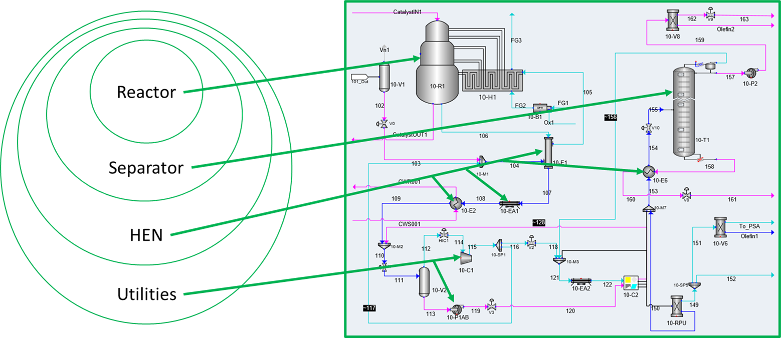
Next, flow rates, vapor/liquid equilibria, temperatures, pressures, and the heating/cooling requirements can be used to design the heat exchanger network (HEN). To complete the design, the auxiliary services or utilities (steam, cooling water, pumps, compressors, etc.) required by the process are determined. Finally, the consumption of these auxiliary services is optimized for operating efficiency.

Changing process design conditions, such as reaction temperature or column reflux ratio, have a noticeable impact on energy and utilities consumption. Using the sequential design approach illustrated in the onion diagram, the impact of process condition changes on energy consumption cannot be identified. Multiple iterations between process design and the corresponding utility system design steps are required to fully capture the potential for energy savings, and this procedure is called process optimization.

How the software is applied is as important as the software itself – this is true for tasks ranging from basic line sizing simulators to complex integrated simulation and economic evaluation packages. Fortunately, software is increasingly user-friendly and intuitive, often featuring guided examples with multiple levels of complexity. Regardless of developer, most process simulation software products utilize several common general procedures and practices, and this article explores the most important principles for using software to generate accurate simulation models.

Selecting a Thermodynamic Property Package

There are two traditional classes of thermodynamic models for phase equilibrium calculations: 1. liquid activity coefficient models, and 2. equation-of-state models. Activity coefficient models can be used to describe mixtures of any complexity, but only as a liquid well below its critical temperature. An equation of state – typically empirical in nature – is any mathematical relation between volume, pressure, temperature, and composition, and most forms of these equations are of the pressure-explicit type. The simplest useful polynomial equation of state is cubic, for such an expression is capable of both yielding the ideal gas equation as volume goes to infinite and representing liquid- and vapor-like molar volumes at low temperatures. These cubic parameters are constrained to satisfy the critical conditions, and as a result these equations can provide an exact duplication/prediction of the critical pressure and temperature which is the end point of the vapor pressure curve.

Another important feature in these equations is the inclusion of a term that can be adjusted to provide an accurate description of the vapor pressure of any polar or nonpolar components from the triple point to the critical point. The success of calculating vapor-liquid equilibrium data also depends on the mixing rules upon which the accuracy of predicting mixture properties relies.

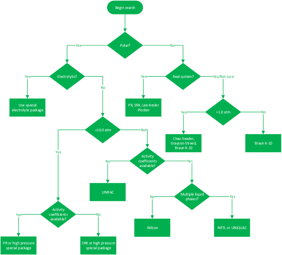
The following flow diagram can be used to help decide which activity coefficient model or equation of state should be used to get accurate results from a simulation model.

Additional guidance regarding these two types of thermodynamic models is as follows:

• Activity coefficient models
  • Can be flexible and able to fit complicated vapor-liquid equilibrium (VLE) and liquid-liquid equilibrium (LLE).
  • Good approximations for activity coefficient values can be generated using UNIFAC.
  • Majority of the time, temperature-dependent interaction parameters are required.
  • Density, enthalpy, entropy, and heat capacity should be calculated by a special correlation and not by the used activity model.
• Equations of state
  • Simple, fast, and consistent across the mixture critical point for hydrocarbons.
  • Good results for certain classes of problems (e.g., refining and gas processing).
  • Can be used with minimum experimental data.
  • Other physical properties can be calculated accurately (e.g., density, enthalpy, entropy, heat capacity, etc.).
  • Liquid density results are not accurate enough for process design.
  • For pure components, the critical properties and acentric factor are required to calculate vapor pressures.
  • Provide a good estimate of water in the hydrocarbon phase, but not of hydrocarbon in the water phase, and commonly predict an incorrect phase split.

Setting Up and Running Process Simulations

Process simulations are essentially a series of heat and material balances combined with process equipment models and thermodynamic property packages. Here are some useful guidelines:

• Always start from the feed, proceed to the main product, and prioritize the main flow path to be solved first.
• Define a calculation sequence for the simulation.
• If a recycle stream is required, estimate initial values within a reasonable operation range for pressure, temperature, flow, and composition. This is critical to ensuring that all recycle stream information is propagated through the system before the recycled stream values are determined.
• Always have a clear understanding about the simulation’s degrees of freedom.
• It is recommended to isolate particularly complex sections and/or unit operations from the main simulation. These can be solved and optimized separately, and then (re)integrated once they are properly arranged.
• Use experimental design and analysis techniques to build and improve designs. Run multiple “case studies” with different process equipment and flow settings, so the generated information can be qualitatively and quantitatively analyzed.
• Only use real and experimental information to estimate initial parameters.
• Set reasonable parameters for the numerical method used to converge the simulation model (e.g., minimum and maximum values, iteration step, and tolerances).
• Always ensure the thermodynamic property package being used is suitable for the mixture and test/compare the calculated results against known experimental data.
• Frequently check and use the software user manual.

Steady-State Simulation

A steady-state simulation is useful to establish heat and material balances and compositional information, thus providing an estimate of long-term process equipment performance and raw material and utility requirements. However, because they disregard the parameter time, steady-state simulations can only simulate continuous processes and not simulate nonlinear processes (e.g., startups, emergency shutdowns, scalability scenarios, etc.).  In addition, keep the following in mind:

• Be aware of all the logical unit operations included in the software (e.g., controllers, adjusters, sets, spreadsheets, monitors, etc.) that will help to run the case studies. This is critical to ensure a good convergence of the simulation.
• The software is not sufficiently intelligent to recognize unreasonable operating parameters.
• It is recommended to use heat loss correlation if available, as in reality there are no adiabatic or no heat-transfer processes.

Dynamic Simulation

Whereas steady-state simulation solves a single point, a dynamic simulation solves a series of single points. Each point is separated in time by the step size. Steady-state simulations solve and converge unit operations/recycle streams one at a time and follow a defined calculation sequence; in a dynamic simulation, pressures and flows are solved simultaneously using a network solver, and energy and composition balance are determined on a per unit operation basis. This allows for the analysis of time-sensitive simulations such as start-up and shutdowns, nonlinear systems, and noncontinuous processes, and it is critical to creating and defining process control schemes. Some specific guidelines for dynamic simulation are as follows:

• Choose the correct specifications for dynamic simulation, such as pressure rather than mass flow for boundary streams, geometry (e.g., length, diameter, or volume) for nodes like separators, and area constant (e.g., Cv, orifice area, internal diameter, etc.) for flow resistances like control valves or pipes. For rotating equipment, the required specifications are head, efficiency, and speed.
• Revise the numerical integration method and parameters for suitable model convergence.
• Specify a reasonable step size before running the simulation. Consider decreasing the step size if the integrator fails to converge, and increase it when the simulation is stable. If the simulation includes many pure components or hypothetical components always start with a very small step size under the range of 0.1 – 0.25 s. Note that a larger number of components increases the complexity of the compositional calculations and slows down the simulation solver.
• Dynamic simulation is more time-consuming than steady-state simulation and requires a well-defined calculation sequence.
• Flow rates in and out do not match because of inventory volumes in process equipment.
• Temperatures, pressures, flow rates, and levels are regulated by defined control loops. These control loops require calibration of the controller unit operations, and it is mandatory to review the proportional gain ratio constant, integral time constant, derivative time constant, mode, and action of the controller before running the model for stable control of the simulation.
• Use stripcharts to fully understand the behavior of multiple profiles through time.
• Pay attention to specific correlations and parameters in the different process equipment, including:
  • Piping – friction loss and heat loss
  • Heat exchangers – heat-transfer coefficient and pressure drop
  • Separators – heat loss and entrainment
  • Rotating equipment – flow basis and calculation type for performance curves
  • Distillation columns – mass-transfer coefficient, efficiency type, and pressure drop
  • Ideal reactors – simultaneous reactions and reaction kinetics

Optimizing the Process

After a process is simulated and converged, it is time for process optimization. An optimum design is developed by determining the objective function that is to be maximized or minimized as well as the structural and parametric variables and constraints that affect the objective function. Variables and constraints can include total cost per unit of production or per unit of time, profit, amount of final product per unit of time, and percent conversion.  

In defining a well-structured, solvable optimization problem, the following steps are recommended:

• Identify the objective function:
  • Determine what is going to be optimized (e.g., maximize distillation efficiency, minimize cooling water flow rate, etc.).
  • Formulate the objective function mathematically, taking advantage of the software tools (case study, optimizer, data filter, controller, scheduler, selector block, set, etc.).
• Define the decision variables:
  • Identify the process variables (decision and dependent variables) that can be controlled or adjusted in the optimization process. Decision variables are variables that can be determined or set, while dependent variables (e.g., operating conditions and equipment specification such as number of trays in a column) arise or are influenced by process constraints.
• Establish the process constraints:
  • Identify any process restrictions or limitations on the decision variables (e.g., process operability limits, reaction chemical species dependence, or product purity and production rate).
  • Additionally, identify the type of the process constraints. Define continuous variables, i.e., factors that may vary continuously over a certain range (e.g., temperature and flow rates that can be set to vary smoothly), and discrete variables that are limited to a discrete group of values (e.g., set-position switches).
• Formulate the optimization model:
  • Combine the objective function, decision variables, and process constraints into a coherent mathematical model with the help of logical unit operations available in the software.
  • The most general mathematical models for chemical processes require consideration of gradients in both time and spatial coordinates. Gradients such as composition or temperature can therefore be visualized with up to four dimensions and require the use of partial differential equations for proper mathematical representation.
  • Ensure that the optimization model represents the problem.
• Choose the optimization method:
  • Select the appropriate optimization technique based on the nature of the objective function and process constraints. Multiple numerical methods should be available in the software, such as interior point, Nelder-Mead, Augmented Lagrangian Multiplier, nonlinear interior point, quasi-Newtonian method, Powell, etc.
  • Tune the multiple method parameters so the model runs smoothly (e.g., maximum iterations, tolerance, gradient and Jacobian perturbations, objective function type, etc.).
• Implement the model:
  • Ensure that the implementation can handle the complexity and scale of the optimization problem.
• Solve the optimization problem:
  • Run the optimization model to find the optimal solution.
  • Use tools such as the monitor, historian, plots, etc., to track the performance of the simulation.
• Analyze the results:
  • Evaluate the integrated solution to ensure it meets the objective and adheres to all process constraints.
  • Perform sensitivity analysis to understand the impact of changes in decision variables and process constraints (continuous and discrete).
• Iterate if necessary:
  • If the solution is not satisfactory, refine the optimization model, adjust constraints, or reconsider the objective function.
• Document the optimization process and results:
  • Keep detailed records of the optimization process, assumptions, and results.
  • Ensure that the documentation is clear and comprehensive for future reference or validation.
  • Always save the simulation before running with a different name; in case the solution is not suitable, there will be an initial model to modify.

These steps are derived from general optimization principles and specific methodologies discussed in various sources, including the use of penalty functions for transforming constrained problems, the importance of defining clear constraints and objective functions, and the application of optimization techniques in structural design. Following this general guidance for using process simulation software will support maximum efficiency at the lowest practical cost.

References

• A. Rutherford, Mathematical Modeling: A Chemical Engineer’s Perspective, Academic, 1999.
• E.F. Camacho and C. Bordons, Model Predictive Control, Springer-Verlag, 2000.
• L.T. Biegler, I.E. Grossman and W. Westerberg, Systematic Methods of Chemical Process Design, Prentice-Hall, 1997.
• Symmetry Process Simulation Platform user’s manual, 2025.
• B. Linhoff, A User Guide on Process Integration for the Efficient Use of Energy, Gulf Publishing, 1994.
• I. C. Kemp, Pinch Analysis and Process Integration, Butterworth-Heinemann, 2015.

Please submit the form below with any questions for the author: